Thursday, August 11, 2016

Statefarm - experiment 3 - VGG16 finetune


VGG:   [conv(x2/3)->max-pool]xfew-times Then classifier head (4096->4096->1000)

Finetune VGG16

I saw one approach , with great results(!) where the the whole model was loaded, and only the last softmax layer was changed from the original(1000) to the new target (10).
In that case finetuning was done on ALL the model together, with slow learning-rate (sgd 1e-4)

I will use another approach:
We will replace the whole classifier head (4096->4096->1000).
1. [optional to save time later]  Load the model without the last dense part. Run it once on all the images and save to disk all the intermediate output  (512x7x7) per image of the train/validate/test info.  for reference, 10K files should take 1.9 GB of disk space.

2. Create alternative classifier. I used a small one due to a bit weak machine.   256->10
    model = Sequential()  
    model.add(Flatten(input_shape=(512,7,7)))
    model.add(Dense(256, activation='relu'))
    model.add(Dropout(0.5))
    model.add(Dense(10, activation='softmax'))

Train it. I used few optimizers
SGD(lr=1e-3, momentum=0.9, nesterov=True)

SGD(lr=1e-3, momentum=0.9, nesterov=False)- BEST: Saved model to disk vgg_head_only1_out_0_epoc20

SGD(lr=1e-4, momentum=0.9, nesterov=True)

SGD(lr=1e-4, momentum=0.9, nesterov=False)

'adam'


Thursday, August 4, 2016

segmentations

The main two segmentation types are:
semantic-segmentation : color the entire image with a color per class type (usually up to 10 classes like road,cars,pedestreians etc). If there are 3 cars overlapping, we will just see all of them with same color.
Implementation is, usually done in one feed-forward using one softmax on the final layer
see U-Net /SegNet / DeepLab / PSPNet and here

instance-segmentation: color each instance seperatly, even if they are of the same class (3 cars should have 3 masks).
The usual implementation is a first sweep for object-proposals, and then refining each image-patch in a second sweep. Using multiple heads, you can get later bounding-box/classification/human joints key-points, of each image-path. Thus it is, usually, slower than semantic-segmentation.
notable architectures:  r-cnn / fast r-cnn / faster r-cnn / mask r-cnn and  deep-mask/ sharp-mask / multipath-net.  Yolo has another approach.


DeepMask  "Learning to segment object candidates" is below.
I want to also mention new extension to DeepMask, which build on it and improve.
SharpMask "Learning to refine object segments" - better attempt:  really good  article!! which both improve the speed to DeepMask itself and then adds architecture on it.
A MultiPath Network for Object Detection


Object detection and Object proposals.
Object detection is one of the most foundation tasks in computer vision, unlike classification which say what is the main object somewhere in the image, object-detection it needs to find multiple objects in the scene, and their exact location bounding-box or even their pixel-mask.
The usual CNN architectures are good at returning one object classification and/or one location, but not multiple ones in one sweep.
Until recently, the dominant paradigm in object detection was the (dumb) sliding window framework: a classifier is applied at every object location and scale, which means running it a-lot of times.
More recently, Girshick et al. [10] proposed a two-phase approach R-CNN. First, a rich set of object proposals (i.e., a set of image regions which are likely to contain an object) is generated using a fast (but possibly imprecise) algorithm. Second, a convolutional neural network classifier is applied on each of the proposals. This approach provides a notable gain in object detection accuracy compared to classic sliding window approaches. Since then, most state-of-the-art object detectors rely on object proposals as a first pre-processing step [10, 15, 33].


DeepMask goal: Given an input image patch, our algorithm generates a class-agnostic mask and an associated score which estimates the likelihood of the patch fully containing a centered object (without any notion of an object category. In other words, it's a binary-classifier of "something is in the center of the region" and not "it's a horse" or "it's a ball").


The core of our model is a ConvNet which jointly predicts the mask and the object score. A large part of the network is shared between those two tasks: only the last few network layers are specialized for separately outputting a mask and score prediction

Input:
image-patch
label binary classfier : 1 or -1 , if object is fully contained, and centered in the patch.
label: mask:  1 or -1 on all the pixels, only relevant if label exist


Architecture:
Based of VGG-A  (8 conv layers, 5 polling layer) without the last pooling layer and dense-head.  They also use pre-trained weights.  Meaning 4 max-polling which take 3xWxH image and make it 512 x W/16 x H/16. look at the image for the different heads.
Note that in the seg-branch there are no activation (no 'relu' or other)

Joint-loss: 
Smartly defined as 
score_constant * binary log-loss on the score (1/-1) 
+ (Yscore+1)/path-size * sum of binray log-loss per pixels

We alternate between backpropagating through the segmentation branch and scoring branch (and set score-constant to  1/ 32 ).
For the scoring branch, the data is sampled such that the model is trained with an equal number of positive and negative samples. Note that the factor multiplying the first term (Yscore+1)implies that we only backpropagate the error over the segmentation branch if yk = 1. In other words, the segmentation is learning only on real-objects and at test time, we ignore it's input otherwise.

Full-scene
Go over all the image in strides of 16 pixels.  Some trick is used (Read the paper). Test multiple patches each time


Implementation Code

unofficial-implementation in keras
Let's discuss some non-trivial points.

combined-loss
Here we have one combined loss function for two classifier-heads, which can't work in parallel as if the classifier-head decides there is no object, the segmentation-head output is ignored, we do not back-propagate loss from that head.
Here is a workaround. there is a request for change on thgis multi-target-loss
Another trick (more of a hack) if to use dirty-pixel , like the upper-left which will mark what we have.

def binary_regression_error(y_true, y_pred):
    return score_output_lambda * K.log(1 + K.exp(-y_true*y_pred))

def mask_binary_regression_error(y_true, y_pred):
    trick = 0.5 * (1 - y_true[:,0,0])  # for Batch of 3, will where one is negative will be [0,1,1]
    #note: the mean is per batch K.sum [0,1,1] * [0.33, 0.33 , -0.333] (the mean of 3 batches)
    #also note that it's not normailized between different batches( some can be all zeroes)
    return trick * K.mean(K.log(1 + K.exp(-y_true*y_pred)),(1,2))

If the absolute value of one brach loss is much-higher than the other, we will not "learn" in the other bracnh. In the article, they specify they alternated between propogating the branches.
One can simply change the "strength" of the loss each round (and then recompile)
score_output_lambda = 1 if round_number%2==0 else min_score_output_lambda


SharpMask

First, faster , better DeepMask, by using resnet instead of VGG, and by changing the classification heads to 128x1x1 conv (output: 128x10x10) tensor-> 512x1x1 tensor.  Split to:
Score:  add 1024x1x1  then 1x1x1 score
Segmentation:


Monday, July 18, 2016

Statefarm - experiment 2

Use pre-trained googlenet.
Step 1: get a pre-training googlenet
Find one on the net , usually converted from caffe model. make sure you understand how to pre-process the data , by testing few images.

Step 2: Cut it's head classifier and replace it with yours. Then train your new classifier on the frozen body (the no-head part).
googlenet classifier has 1000 categories, and there are actually 3 heads to the body - a "hydra" :)
There is a main one and 2 aux classifiers in the middle. All need to be replaced and trained.

This is the graph of the main-classifier trained, while all the rest of the model is frozen (in-fact, I dumped to file the output of the 'merge' layer prior to the classifiers sections, it saved a lot of time, but cost few dozen of Gigs of disk space)
After 12 (model_chapter6_12epoc) , we don't see any increase.  This is the output of 32:
loss: 0.5412 - acc: 0.8648 - val_loss: 0.9205 - val_acc: 0.6908

In the same way, we will train the other 2 aux classifiers. aux1 (middle one)

  loss: 0.1330 - acc: 0.9771 - val_loss: 1.2633 - val_acc: 0.8178
Saved model to disk model_chapter6_aux1_try2_11epoc

aux0 - behaves surprisingly well (look at the wierd behaviour of the validation - higher than the training in epoc1. then going down...

loss: 7.4296 - acc: 0.3291 - val_loss: 0.4846 - val_acc: 0.8513
Saved model to disk model_chapter6_aux0_1epoc

loss: 0.1624 - acc: 0.9737 - val_loss: 0.5066 - val_acc: 0.9082
Saved model to disk model_chapter6_aux0_8epoc

Even without fine-tuning, we might use the aux0 for validation loss of 0.5, or the other classifiers for 0.9/1.2 loss.
Let's test this and submit the model with aux0
(used model_chapter6_aux0_25epoc)
Validation score= 0.1 accuracy= 0.92
LeaderBoard: 1.82
Conclusion: Classic case of overfit to the validation. So let's continue to step 3

Step 3: connect the new heads and fine-tune the entire model. 
We will do it by freezing most layers (the inception-blocks), except the last one/two blocks.
We will use the new classifier. 
Note on this quite "low" number -
  • We did not augment the data while training this
  • We used rmsprop which is a "fast but less accurate" one.
We did this, as we will have a training step later, which should work with augmentation and better optimization.


3.1 bad-experiment example (eveyone have bugs...)
Use only partial graph (only the aux0). high learning rate 0.001. heavy augmentation (flip/zoom/shear). Can you see the problem here?


This should never happen, and is usually a bug.  The bug in this case was in bad-random flip (on training always flip . on validation never flip)
result in: model_chapter6_aux0_finetune7epoc

3.2 Can we use only aux0 and a small subset of the googlenet?  (the answer is no...)
We again only partial graph with aux0, this time slower learning rate of 0.0001
result sample in: model_chapter6_aux0_finetune_lr_1e40epoc This proved to be have bad results

3.3 Let's finetune the whole model, and look the the result of the end-classifer. fine tuned 16 epocs using SGD 0.003 This proved to be great improvement, LB=0.51286
lock the first layers: conv1, conv2, inception_3a/b, inception_4a , loss1
keep the other trainalbe: inception_4b/c/d/e inception_5a/b and loss2/3 compile while adding loss_weights and add weight to the main classifier: full_model.compile(loss='categorical_crossentropy',loss_weights=[0.2,0.2,0.6], optimizer=SGD(lr=0.003, momentum=0.9), [stopped in the middle] augmentation used: googlenet_augment shift 0.05 rotation 8 degrees, zoom 0.1, shear 0.2
saved model after 16 epocs: model_chapter6_finetune_all_lr_1e4_binary
see: statefarm-chapter6-finetune-0.003-fix_aug.ipynb

validation score (overfit again) SCORE= 0.0529023816348 accuracy= 0.908552631579 confusion matrix:
[[291   0   4   1   1   0   0   0   4  24]
 [  1 298   0  19   0   0   4   0   0   0]
 [  0   0 315   0   2   0   0   0   1   0]
 [  0   1   0 317   0   0   1   0   1   0]
 [  0   0   1   2 313   0   0   0   0   0]
 [  0   0   0   0   0 321   0   0   0   0]
 [  0   0   1   0   0   0 318   1   0   0]
 [  0   0   0   0   0   0   0 256   0   0]
 [  0   0   7   0   0   0   1   1 243   2]
 [156   0   0   0   5   0   1   0   1 125]]
                                precision    recall  f1-score   support

              0 normal driving       0.65      0.90      0.75       325
             1 texting - right       1.00      0.93      0.96       322
2 talking on the phone - right       0.96      0.99      0.98       318
              3 texting - left       0.94      0.99      0.96       320
 4 talking on the phone - left       0.98      0.99      0.98       316
         5 operating the radio       1.00      1.00      1.00       321
                    6 drinking       0.98      0.99      0.99       320
             7 reaching behind       0.99      1.00      1.00       256
             8 hair and makeup       0.97      0.96      0.96       254
        9 talking to passenger       0.83      0.43      0.57       288

                   avg / total       0.93      0.92      0.92      3040

This is the confusion matrix of aux1 classifier (the intermidiate one)
Validation SCORE= 0.0607746900158 accuracy= 0.899342105263
LB score: 0.768
comparing the two confusion-matrixes, 0 and 9 classes
[[191   0  16   4   7  10   1   0  14  82]
 [  0 309   0   5   0   0   7   1   0   0]
 [  1   0 314   0   1   1   0   0   1   0]
 [  0   1   0 312   0   5   0   0   0   2]
 [  4   0   8   5 299   0   0   0   0   0]
 [  0   0   0   0   0 321   0   0   0   0]
 [  0   0   0   1   0   0 316   0   2   1]
 [  1   0   1   0   0   0   0 246   0   8]
 [  0   0   0   0   0   0   0   0 254   0]
 [ 57   0   0   0   5   2   3   0   2 219]]
                                precision    recall  f1-score   support

              0 normal driving       0.75      0.59      0.66       325
             1 texting - right       1.00      0.96      0.98       322
2 talking on the phone - right       0.93      0.99      0.96       318
              3 texting - left       0.95      0.97      0.96       320
 4 talking on the phone - left       0.96      0.95      0.95       316
         5 operating the radio       0.95      1.00      0.97       321
                    6 drinking       0.97      0.99      0.98       320
             7 reaching behind       1.00      0.96      0.98       256
             8 hair and makeup       0.93      1.00      0.96       254
        9 talking to passenger       0.70      0.76      0.73       288

                   avg / total       0.91      0.91      0.91      3040


What will happen if we average the 2 results?
nothing fancy, just simple average of all improves to 0.419 (!)


other results of open competitors
ensamble of VGG16 (0.27) + googlenet (0.38)  together are generate:  0.22
adding-small-blocks from other images , helped a bit more.


Appendix
Looking at some results:

Running few experiment, I constantly get bad results for some of the classes. This is the report:
precision recall f1-score support
              0 normal driving       0.74      0.80      0.77       325
             1 texting - right       0.99      0.97      0.98       322
2 talking on the phone - right       0.95      0.91      0.93       318
              3 texting - left       0.79      0.99      0.88       320
 4 talking on the phone - left       0.98      0.94      0.96       316
         5 operating the radio       0.96      1.00      0.98       321
                    6 drinking       0.96      0.96      0.96       320
             7 reaching behind       0.99      1.00      0.99       256
             8 hair and makeup       0.87      0.92      0.89       254
        9 talking to passenger       0.89      0.59      0.71       288

                   avg / total       0.91      0.91      0.91      3040


The recall for "9-talking to passenger" is extremely bad. (0.59)
The precision for "3 - texting left" is 0.78
and both the precision and recall for "0-normal driving" are bad 0.74/0.80

Let's have a look at some photos, from these categories:
category 0:  
The driver has , usually 2 hands on the wheel, with the head straight ahead, or slightly tilted twards the camera. bad-classification exists, usually when driver looks hard to the right side(probably '9" cattegory)
category 0:  In total 2076 good. 94 bad-human-classification.  4.3% bad classification.

cateogry 9: In total 1364 good. 477 bad-human-classification . 26% (!) bad classification. Mainly drivers looking forward (class "0").  

categoty 3: 
Goog ground truth: rarely right-hand completely shadows the phone (or at least 90% of it). sometime users look cokletely to he right (passenger side), but still, always have a phone.
So why do we have texting-left percision :0.79? let's look at the confusion matrix, we see there are 30 predictions where it was actually class 0


conclusions so far:
Remarkably bad groud-truth classificaiton on category 9 was (according to forum entry) due to classification by whole video-section instead of individual frames.
This means that if in a 30 seconds video, the user did 75% of the time action 9, and 25% of the time action 0, all 100% will be counted as action 9 in the groud-truth.

In other words, there is no way (even a human) can classify it correctly above 75%.
There are two options here:
1. Hack : Reconstruct the video from single-frames, classify the whole section and mark accordingly. 
2. Understand that class 0 can mean both 0 and 9, and artificially change final weights accordingly to minimize error rate


Wednesday, July 13, 2016

ConfusionMatrix

Let's look at one experiment confusion-matrix

[[259   0   7  30   1   8   0   0   7  13]
 [  1 311   0   8   0   0   2   0   0   0]
 [  3   0 288   5   1   0   8   0  13   0]
 [  0   0   0 318   2   0   0   0   0   0]
 [  6   0   0  10 297   2   0   0   1   0]
 [  1   0   0   0   0 320   0   0   0   0]
 [  0   0   0   1   0   0 308   0  11   0]
 [  0   0   0   0   0   0   1 255   0   0]
 [  0   0   7   1   0   0   1   3 234   8]
 [ 78   2   1  29   1   4   1   0   3 169]]

The X axis is prediction . the Y axis is true-label (all first row true-label is 0)
Let's have a look at row 0.
259 in [0,0] means true-positive results with correct match.
30 in   [0,3]  means the truths is 0, but we predicted 3
0 in     [0,1] means we don't think (Wrongly) that 0 is 1
in total there 259 correct-predictions are 7+30+1+8+7+13=66 wrong predictions.
259/325 = 0.80  . This is the hit-rate, or the recall rate.
Let's look at column 0.
78 in [9,0] means we predicted 0, although it is actually 9.  This is a biggest-mistake in one cell. 
If we sum all the column, we see total of 1+3+6+1+78=89 false-positive predictions.  in total we are correct in 259/(259+89)= 0.74 of our predictions, this is the precision.

To iterate on recall and precision, what will happen it we change the algorithm to a dump "always return 0" algorithm?  column 0 will be filled with values. All other columns will be empty.
we will get 325 in [0,0] (all true) and the rest of the diagonal is all false.
The recall will be full 1.00 for 0 category  . We always recall correctly this one.  For the rest it will be 0.00
The precision will be very bad 325/3040 = ~ 10%


precision recall f1-score support
              0 normal driving       0.74      0.80      0.77       325
             1 texting - right       0.99      0.97      0.98       322
2 talking on the phone - right       0.95      0.91      0.93       318
              3 texting - left       0.79      0.99      0.88       320
 4 talking on the phone - left       0.98      0.94      0.96       316
         5 operating the radio       0.96      1.00      0.98       321
                    6 drinking       0.96      0.96      0.96       320
             7 reaching behind       0.99      1.00      0.99       256
             8 hair and makeup       0.87      0.92      0.89       254
        9 talking to passenger       0.89      0.59      0.71       288

                   avg / total       0.91      0.91      0.91      3040


Let's analyze back to the classification-report.
about "0 - normal-driving" we talked already.
We can see that "1- texting-right" has good recall 0.97, and also good precision 0.99
'3-texting-left" has 0.99 recall, but only 0.79 precision (it's too-strong) which means there are many false-assumptions, let's look at the confusion-matrix, at column 3. 30 predictions were actually 0-normal-driving and 29 are actually 9-talking-to-passenger.   


True Positive (TP)  eqv. with hit
False Positive (FP) eqv. with false alarm, Type I error


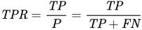
sensitivity or true positive rate (TPR) eqv. with hit rate, recall

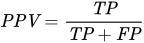
precision or positive predictive value (PPV)

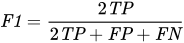
F1 score - is the harmonic mean of precision and sensitivity